


EP16.TOKT11122 · Compulsory
Time Series Analysis and Forecasting
- Credits
- 3
- Lecture
- 30 h
- Lab
- 15 h
- Self-study
- 90 h
1. General information
| Course title | Time Series Analysis and Forecasting |
|---|---|
| Course code | EP16.TOKT11122 |
| Type | Compulsory |
| Credits / hours | 3 credits · Lecture: 30h · Lab: 15h · Self-study: 90h |
| Prerequisites | EP16.TOKT1145; EP16.TOKT11108 |
2. Department and instructor
Department: Faculty of Data Science and Artificial Intelligence, National Economics University.
Address: Suite 1105, Building A1, NEU


3. Course description
This course provides a practical introduction to time series analysis and forecasting with applications in finance, economics, and healthcare. Students use Python (NumPy, Pandas, Matplotlib, Statsmodels, scikit-learn, and optionally deep learning frameworks) to work with real-world time-indexed data.
Core topics include time series concepts and components, exploratory analysis, stationarity, ARIMA and SARIMA models. In the later weeks, students are introduced to machine learning and deep learning methods for time series, such as tree-based models and simple recurrent or convolutional neural networks.
The course is strongly project-based. Students work in groups on real datasets (stock prices, macroeconomic indicators, vital signs, EEG/ECG signals). All lab weeks are dedicated to project progress presentations. A Midterm Project Baseline Report replaces the traditional midterm exam and focuses on establishing strong classical baselines. The final deliverable is a comprehensive group project including both classical and ML/DL methods.
4. Learning resources
Main textbooks
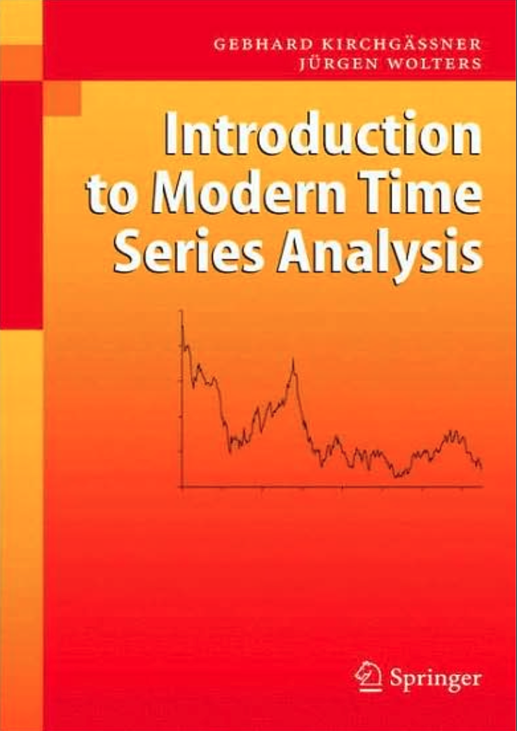
- Gebhard Kirchgässner, Jürgen Wolters (2013). Introduction to Modern Time Series Analysis.
- Springer.
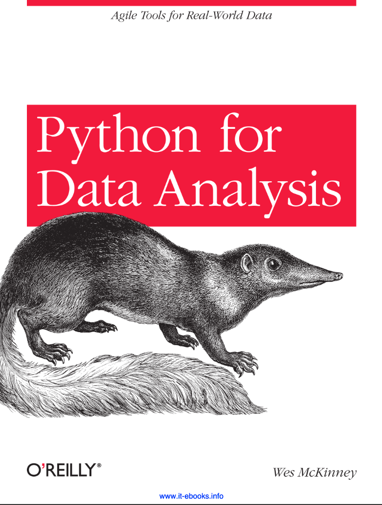
- Wes McKinney (2022). Python for Data Analysis.
- O'Reilly Media.
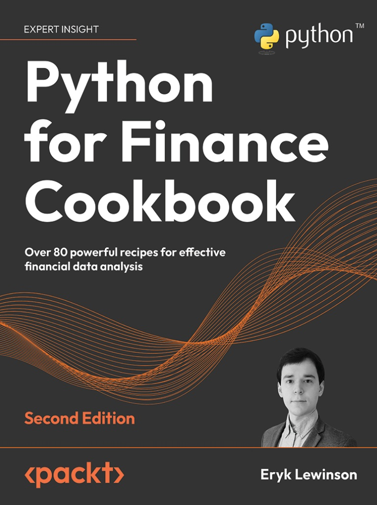
- Eryk Lewinson (2022). Python for Finance Cookbook.
- Packt Publishing.
Other references
- Tarek A. Atwan (2022). Time Series Analysis with Python Cookbook.
- Packt Publishing.
- Changquan Huang, Alla Petukhina (2022). Applied Time Series Analysis and Forecasting with Python.
- Springer.
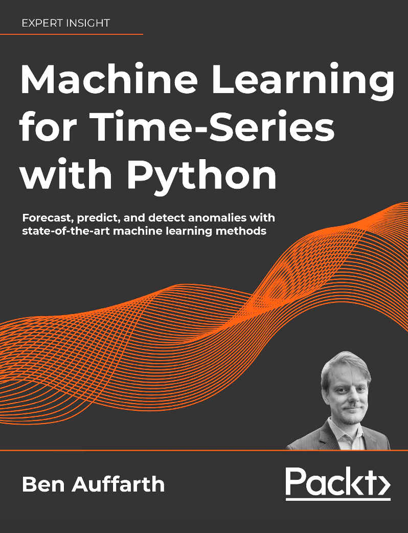
- Ben Auffarth (2021). Machine Learning for Time-Series with Python.
- Packt Publishing.
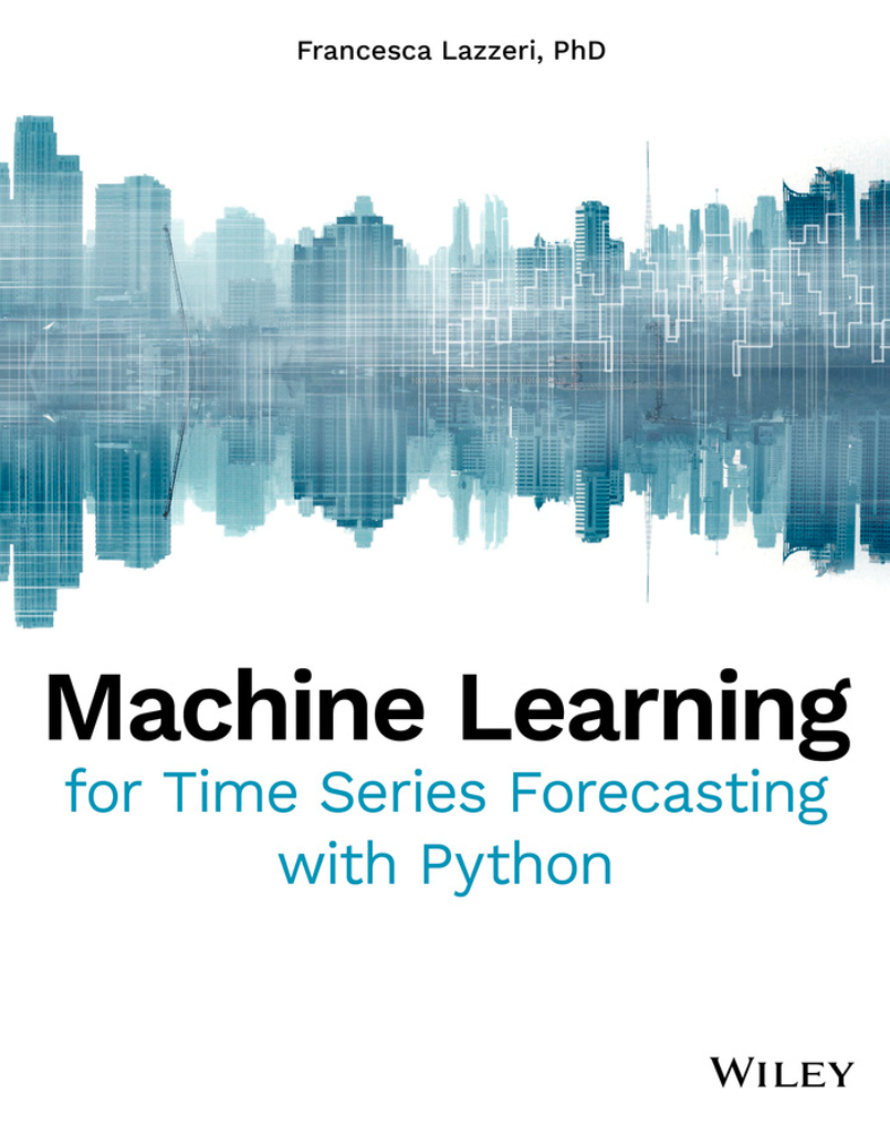
- Francesca Lazzeri (2020). Machine Learning for Time Series Forecasting with Python.
- Wiley.
Online notes: https://online.stat.psu.edu/stat510/
Student Desk
Research Materials & Project Resources
Access the Student Desk for additional resources including:
- Paper and poster templates for project submissions
- Topic notebooks with detailed guidance for each project topic
- Additional research materials and references
5. Course objectives
- G1. Understand fundamental time series concepts and their applications in stock markets, finance, economics, and healthcare.
- G2. Collect, preprocess, and manipulate time series data in Python using appropriate libraries.
- G3. Conduct exploratory time series analysis, including visualization, decomposition, and stationarity assessment.
- G4. Model and forecast time series data using core statistical methods such as ARIMA and SARIMA.
- G5. Apply and compare traditional time series models with basic machine learning and deep learning methods for forecasting.
- G6. Develop teamwork, self-study, independent work, and shared responsibility within project groups through a project-based learning approach.
6. Course learning outcomes
| CLO | Obj. | Outcome |
|---|---|---|
| CLO 1.1 | G1 | Explain key time series concepts (trend, seasonality, cyclicity, noise) and their relevance in real-world applications. |
| CLO 1.2 | G2 | Use Python (Pandas, NumPy, Matplotlib, Statsmodels) to load, preprocess, and visualize time series data. |
| CLO 2.1 | G3 | Perform exploratory analysis of time series using ACF/PACF, decomposition, and smoothing techniques. |
| CLO 3.1 | G3 | Explain the concept of stationarity and apply differencing and basic tests (e.g. ADF) to assess it. |
| CLO 3.2 | G4 | Build and interpret AR, MA, and ARMA models and implement them in Python. |
| CLO 4.1 | G4 | Build, evaluate, and diagnose ARIMA and SARIMA models using the Box–Jenkins methodology. |
| CLO 4.2 | G5 | Transform time series into supervised learning format and implement basic machine learning models for forecasting. |
| CLO 4.3 | G5 | Describe the role of deep learning models (RNN/LSTM/CNN) for time series and implement a simple example. |
| CLO 5.1 | G5 | Design and implement a complete forecasting pipeline on a real dataset, combining classical and ML/DL approaches. |
| CLO 5.2 | G5 | Analyze and interpret model results, compare methods, and provide actionable insights. |
| CLO 6.1 | G6 | Demonstrate self-study and independent work through homework and project contributions. |
| CLO 6.2 | G6 | Collaborate effectively in teams and report project progress clearly in written and oral form. |
7. Course assessment
| Type | Content | Week | CLOs | Tools / Criteria | Weight |
|---|---|---|---|---|---|
| Homework | Theory and programming (individual) | Selected weeks | 1.2, 2.1, 3.1, 3.2, 4.1, 4.2, 4.3, 6.1 | LMS submission; correctness; application to time series; time management. | 20% |
| Midterm Project Baseline | Group baseline report (PDF) + presentation | Week 10 | 1.2–4.1, 5.1, 5.2, 6.1, 6.2 | EDA, ARIMA/SARIMA baseline, forecasts and plots; clarity and structure. | 30% |
| Final Project | Full group project report + final presentation | Week 15 | 1.1–5.2, 6.1, 6.2 | Integration of classical and ML/DL models; depth; comparison; clarity; teamwork. | 50% |
- All lab weeks are used for group progress presentations. These count toward the overall project evaluation (midterm and final), not as separate lab assignments.
- The Midterm Project Baseline replaces a traditional written exam and focuses on producing a strong classical (ARIMA/SARIMA) baseline.
8. Teaching plan (15 weeks)
Lecture and lab weeks alternate. All lab weeks are group progress presentations. Weeks marked TBD are not yet finalized and publish no materials.
| Week | Format | Content highlights | Activities / Assessment | CLOs |
|---|---|---|---|---|
| 1 | Lecture | Intro, project requirements, Python ecosystem, environment setup, Kaggle overview | Lecture, demo, Q&A | 1.1, 1.2, 6.1, 6.2 |
| 2 | Lecture | NumPy review; Pandas for time series; resampling, rolling stats; SMA/EMA/RSI/MACD | Lecture + code walkthrough; Homework 1 | 1.2, 2.1, 6.1 |
| 3 | Lecture | Time series components; ACF/PACF; decomposition; smoothing | Lecture + code examples; Homework 2 | 2.1, 3.1, 6.1 |
| 4 | Lab | Project kick-off; dataset intro; first plots | Group presentations; open lab time | 1.2, 5.1, 6.1, 6.2 |
| 5 | Lab | EDA on project data; trends/seasonality; issues | Group presentations; feedback on modeling direction | 2.1, 3.1, 5.1, 5.2, 6.1, 6.2 |
| 6 | Lecture | Stationarity; unit root tests; differencing; AR/MA/ARMA models | Lecture + examples; Homework 3 | 3.1, 3.2, 6.1 |
| 7 | Lab | Stationarity checks; AR/MA/ARMA on project data | Group presentations; lab exercises | 3.1, 3.2, 5.1, 6.2 |
| 8 | Lecture | ARIMA, Box–Jenkins process, model selection, forecasting | Lecture + worked example; Homework 4 | 4.1, 6.1 |
| 9 | Lecture | Time-series Classification (TSC) | Lecture + notebooks | 4.2, 5.2 |
| 10 | Lecture/Presentations | Midterm Project Baseline submissions and presentations | Midterm Project Baseline — 30% | 1.2–4.1, 5.1, 5.2, 6.1, 6.2 |
| 11 | Lecture | Seasonality, SARIMA structure, seasonal differencing, SARIMA modeling | Lecture + example | 4.1 |
| 12 | Lab | SARIMA refinements; finalize classical models; plan ML/DL phase | Group presentations | 4.1, 5.1, 6.2 |
| 13 | Lecture | Time series as supervised learning; features; tree-based models | Lecture + notebook | 4.2, 5.2 |
| 14 | Lecture | Deep learning basics for time series: RNN/LSTM/GRU/CNN; workflow | Lecture + notebook | 4.3, 5.2 |
| 15 | Lab/Presentations | Final project report; model comparison; insights | Final Project — 50% | 1.1–5.2, 6.1, 6.2 |
Contact
Questions about the course or projects? Reach out anytime.
Email: nghiant@neu.edu.vn
Website: http://nghianguyen7171.github.io/