Time Series Problem Set: Autocorrelation Function (ACF)

Problem Set (Without Solutions) - Undergraduate Level

Calculation Guide: Mean, Variance, Autocovariance, and ACF

Use the formulas and code below as a reference when computing statistics by hand or checking your work. For a sample time series x₁, x₂, …, xₙ of length n:

Sample mean

x̄ = (1/n) Σᵢ xᵢ

Sample variance (with n−1 denominator)

s² = (1/(n−1)) Σᵢ (xᵢ − x̄)²

Autocovariance at lag k

For lag k, use the demeaned series (subtract the mean first). With n observations, there are n−k pairs (xᵢ − x̄, xᵢ₊ₖ − x̄).

γ(k) = (1/(n−k)) Σᵢ (xᵢ − x̄)(xᵢ₊ₖ − x̄) (sum over i = 1, …, n−k)

Some texts use 1/n instead of 1/(n−k); be consistent. For this problem set, using 1/(n−k) or 1/n is acceptable as long as you use the same convention for γ(0) and γ(k).

Autocorrelation at lag k

ρ(k) = γ(k) / γ(0)

So ρ(0) = 1 always. Autocorrelation is dimensionless and lies in [−1, 1].

Python: computing mean, variance, and ACF

Example with a small array (replace with your data). For ACF, mean removal is applied.

import numpy as np

def sample_mean(x):
    return np.mean(x)

def sample_var(x):
    return np.var(x, ddof=1)  # ddof=1 gives 1/(n-1)

def autocovariance(x, k):
    """Sample autocovariance at lag k, with mean removal."""
    x = np.asarray(x)
    n = len(x)
    x_centered = x - np.mean(x)
    if k >= n:
        return 0.0
    return np.sum(x_centered[:-k] * x_centered[k:]) / (n - k)

def autocorrelation(x, k):
    """Sample autocorrelation at lag k."""
    return autocovariance(x, k) / autocovariance(x, 0)

# Example: compute for a short series
x = np.array([2, 4, 6, 8, 10])
print("Mean:", sample_mean(x))
print("Variance:", sample_var(x))
for lag in [0, 1, 2]:
    print(f"ACF({lag}):", autocorrelation(x, lag))

Without mean removal (for comparison in Exercise Type 2): use xᵢ and xᵢ₊ₖ directly in the product sum instead of (xᵢ − x̄)(xᵢ₊ₖ − x̄). In code, replace x_centered with x in the autocovariance sum.

Exercise Type 1: Numerical ACF Calculation

Problem 1.1

Given the time series: x = [2, 4, 6, 8, 10]

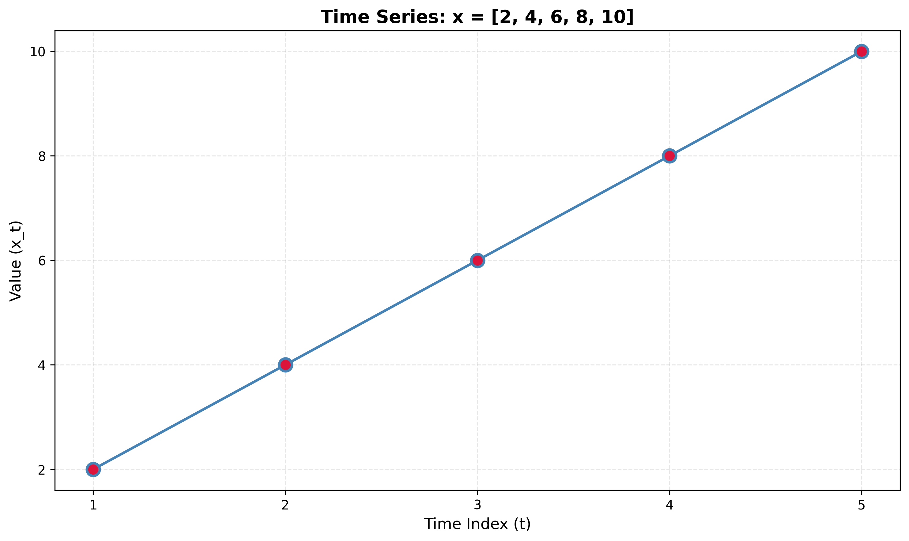
Compute:

The sample mean x̄
The sample variance s²
The autocovariance γ(k) for lags k = 0, 1, 2
The autocorrelation ρ(k) for lags k = 0, 1, 2

Problem 1.2

Given the time series: x = [5, 5, 5, 5, 5]

Compute the autocovariance and autocorrelation. What happens when all values are identical?

Problem 1.3

Given the time series: x = [10, 8, 6, 4, 2]

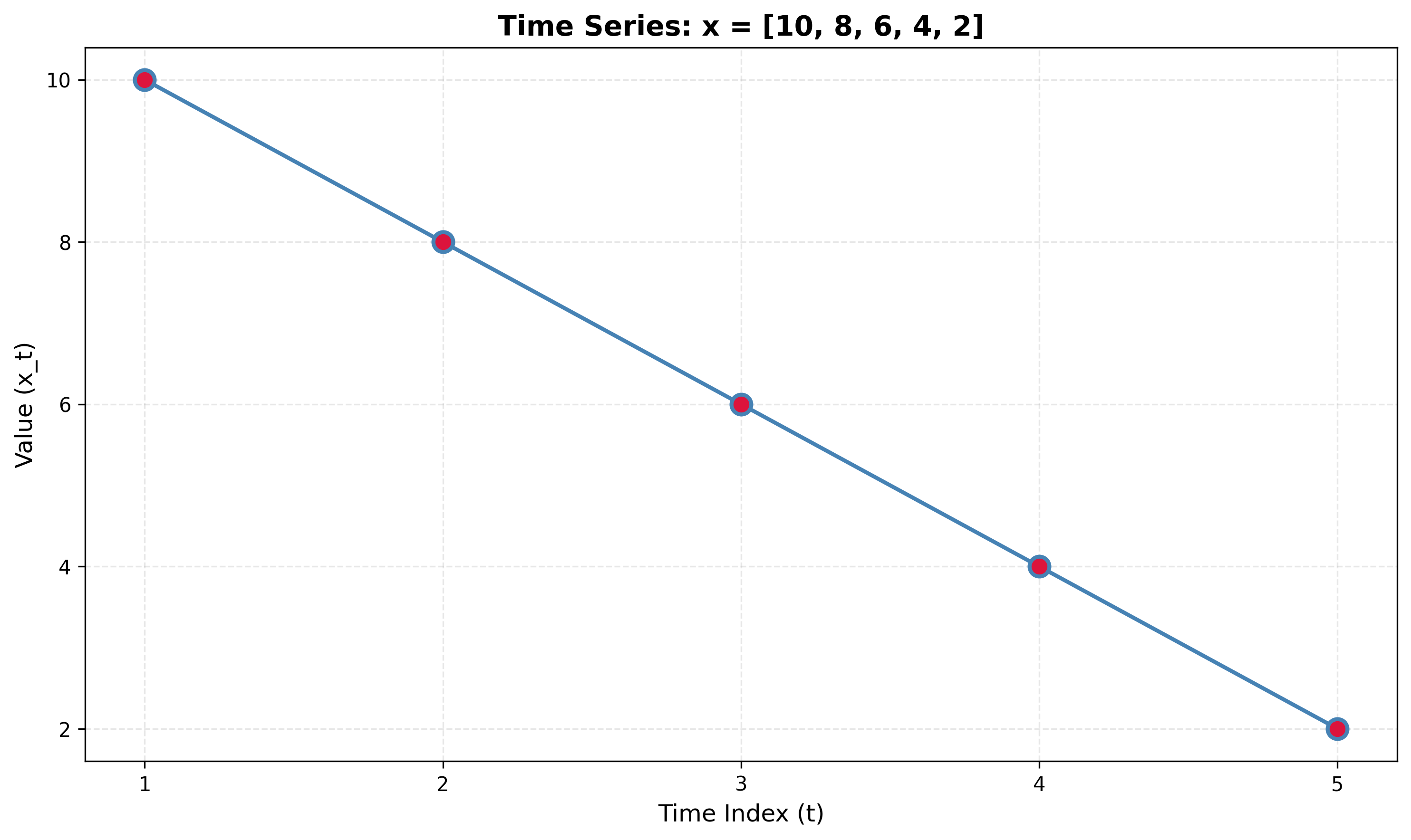
Compute the autocovariance γ(k) and autocorrelation ρ(k) for lags k = 0, 1, 2.

Problem 1.4

Given the time series: x = [3, 7, 3, 7, 3]

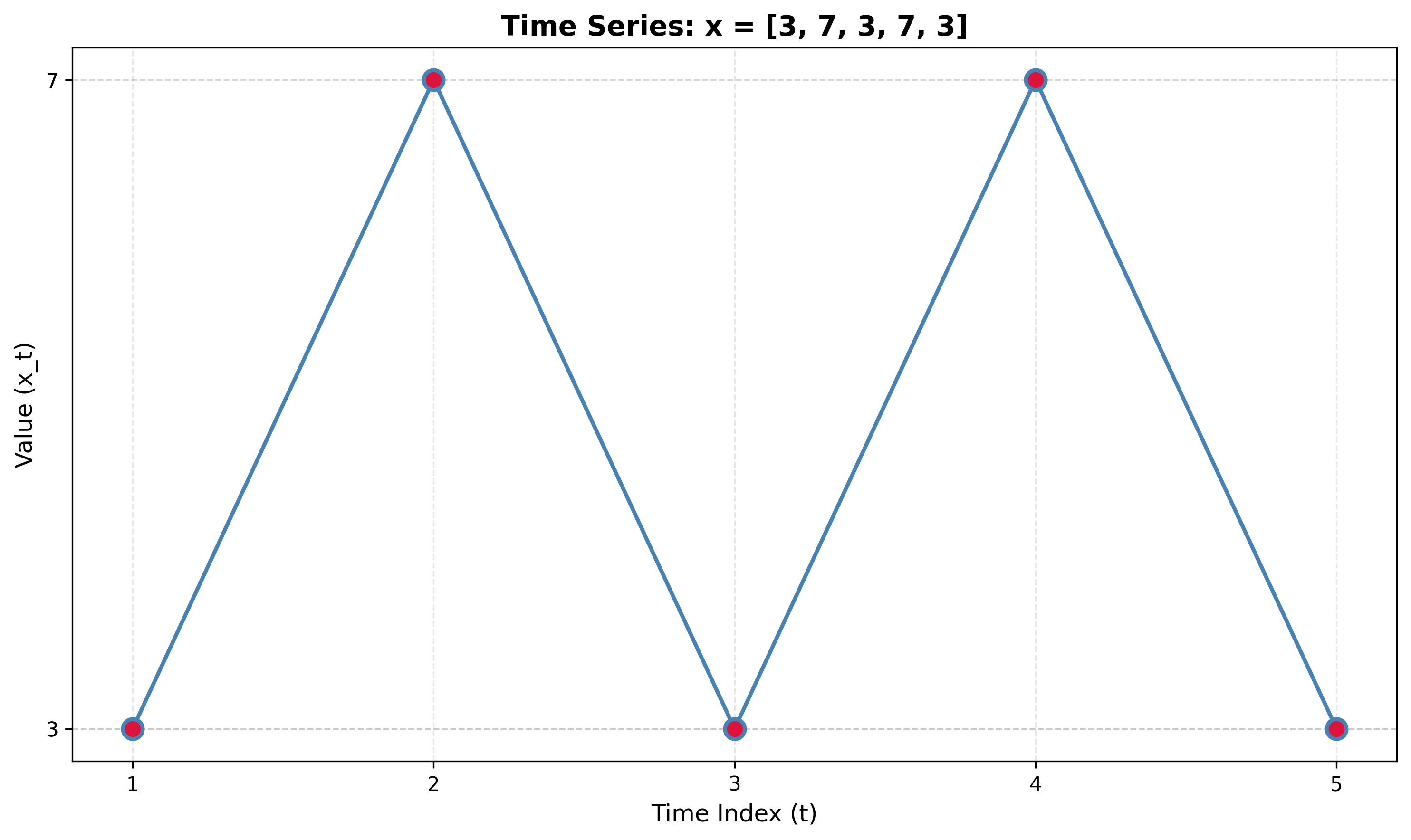
Compute the autocovariance and autocorrelation for lags k = 0, 1, 2, 3.

Problem 1.5

Given the time series: x = [12, 15, 18, 12, 15, 18, 12]

Compute the autocovariance and autocorrelation for lags k = 0, 1, 2, 3.

Exercise Type 2: Effect of Mean Removal

Problem 2.1

Given the time series: x = [5, 7, 9, 11, 13]

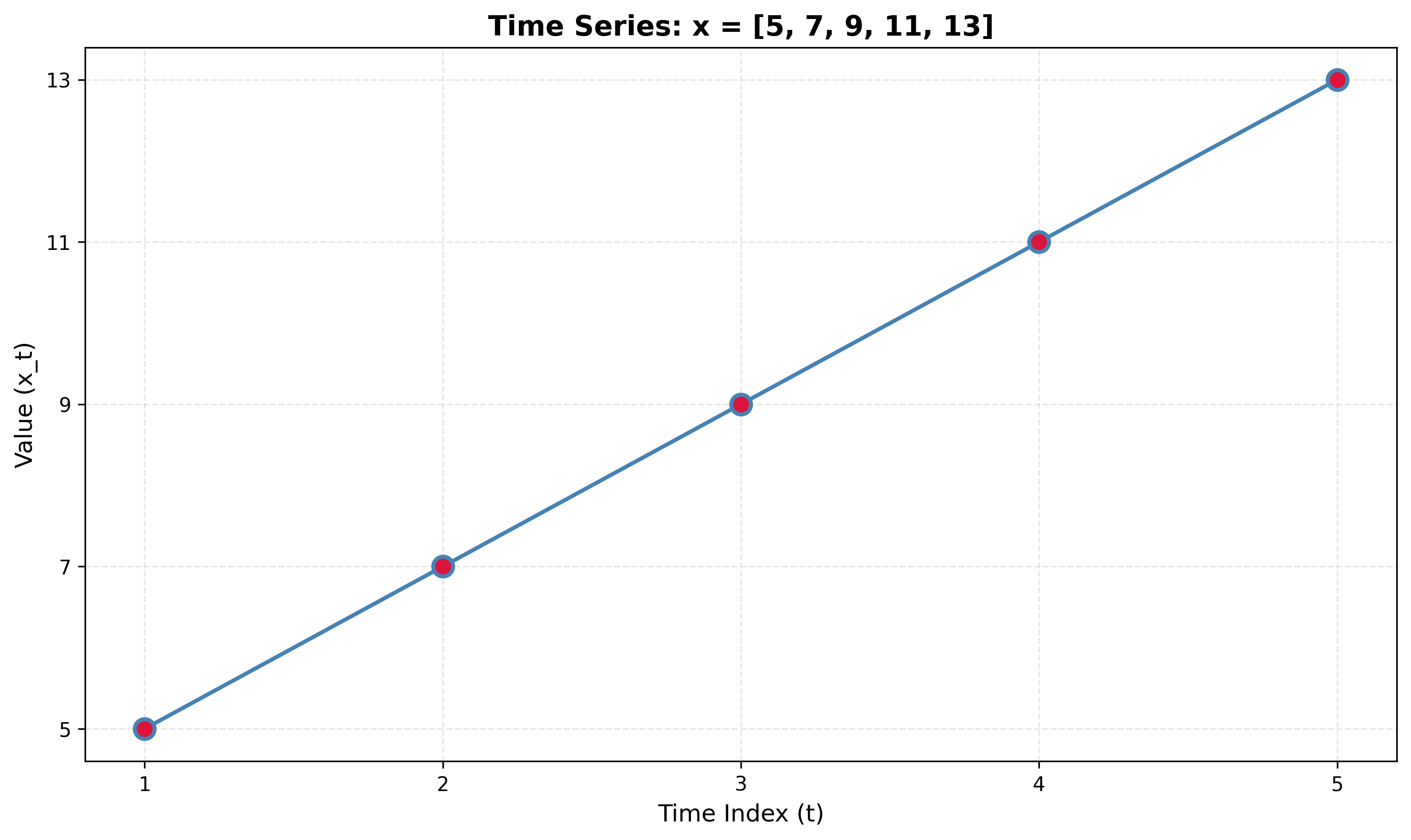
Compute the autocovariance without removing the mean.
Compute the autocovariance with mean removal.
Compare the results and explain why mean removal is necessary.

Problem 2.2

Given the time series: x = [100, 102, 104, 106, 108]

Compute autocorrelation at lag 1 without mean removal.
Compute autocorrelation at lag 1 with mean removal.
Explain the difference.

Problem 2.3

Given the time series: x = [20, 20, 20, 25, 25, 25]

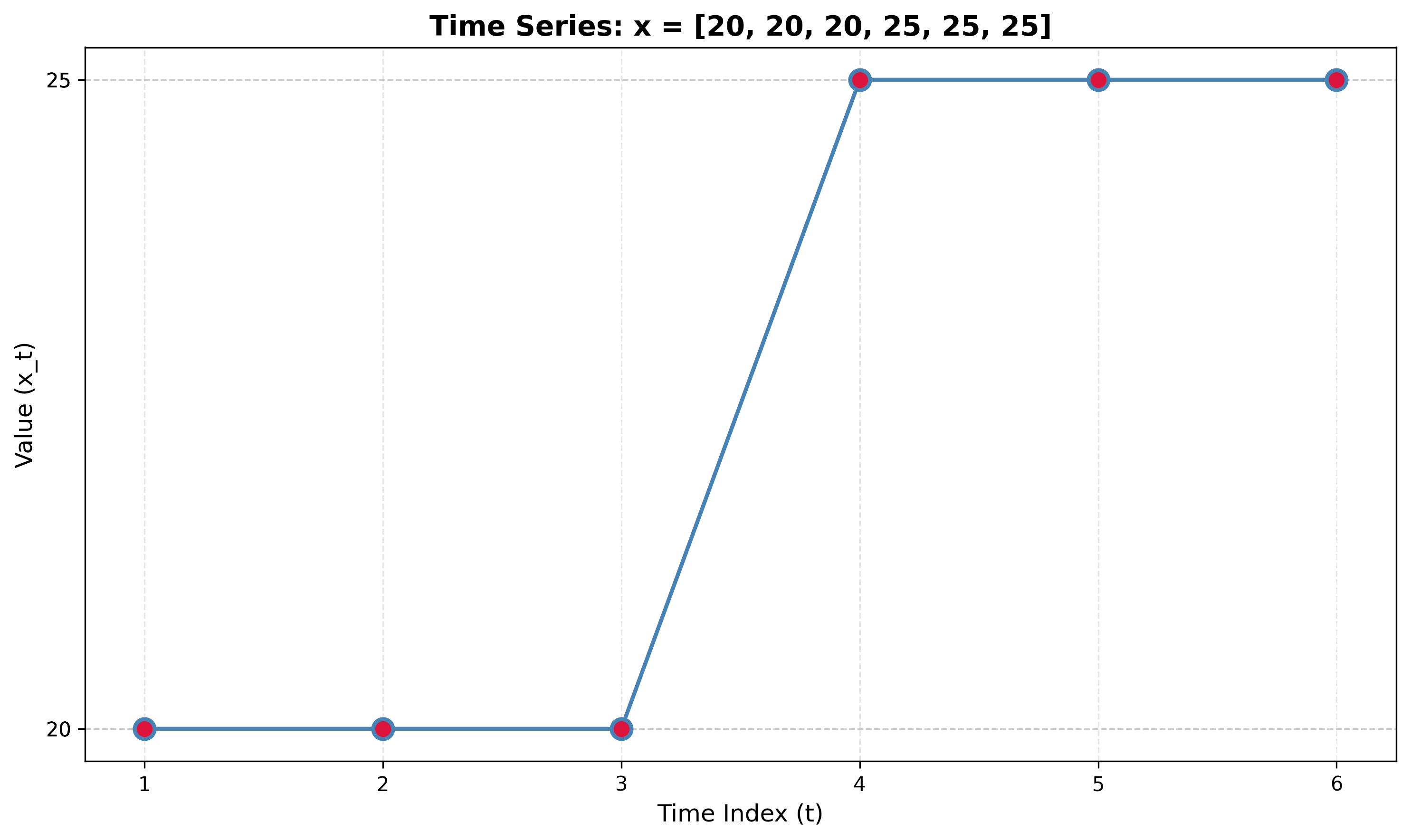
Compare the autocorrelation at lag 1 computed with and without mean removal. What does this tell you about the series?

Problem 2.4

Given the time series: x = [1, 3, 5, 1, 3, 5]

Compute autocorrelation at lag 2 with and without mean removal. Explain why the results differ.

Problem 2.5

Given the time series: x = [10, 12, 14, 10, 12, 14, 10]

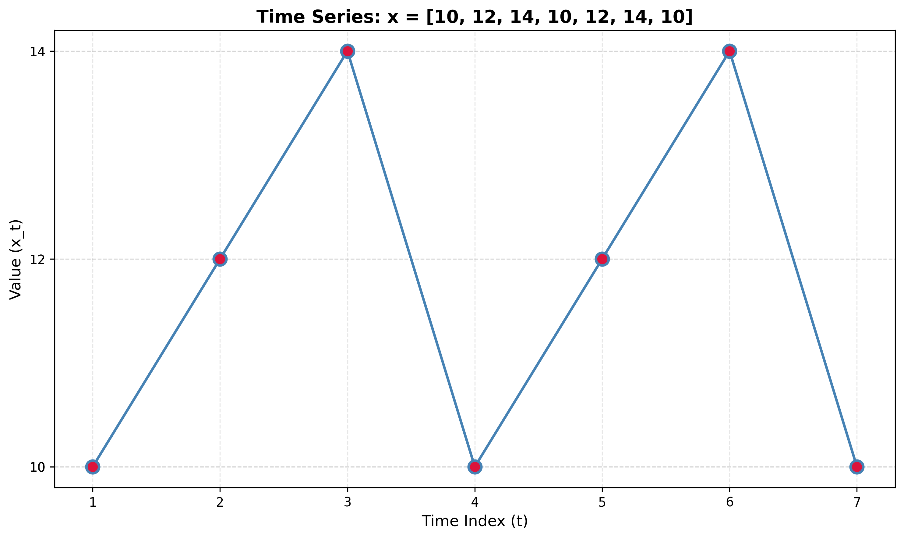
Compute autocorrelation at lag 3 with and without mean removal.
Explain which method gives the correct interpretation of the series' periodic structure.

Exercise Type 3: Interpreting ACF Patterns

Problem 3.1

A time series has an ACF plot where ρ(0) = 1 and ρ(k) ≈ 0 for all k > 0, with values randomly scattered around zero within the confidence bands.

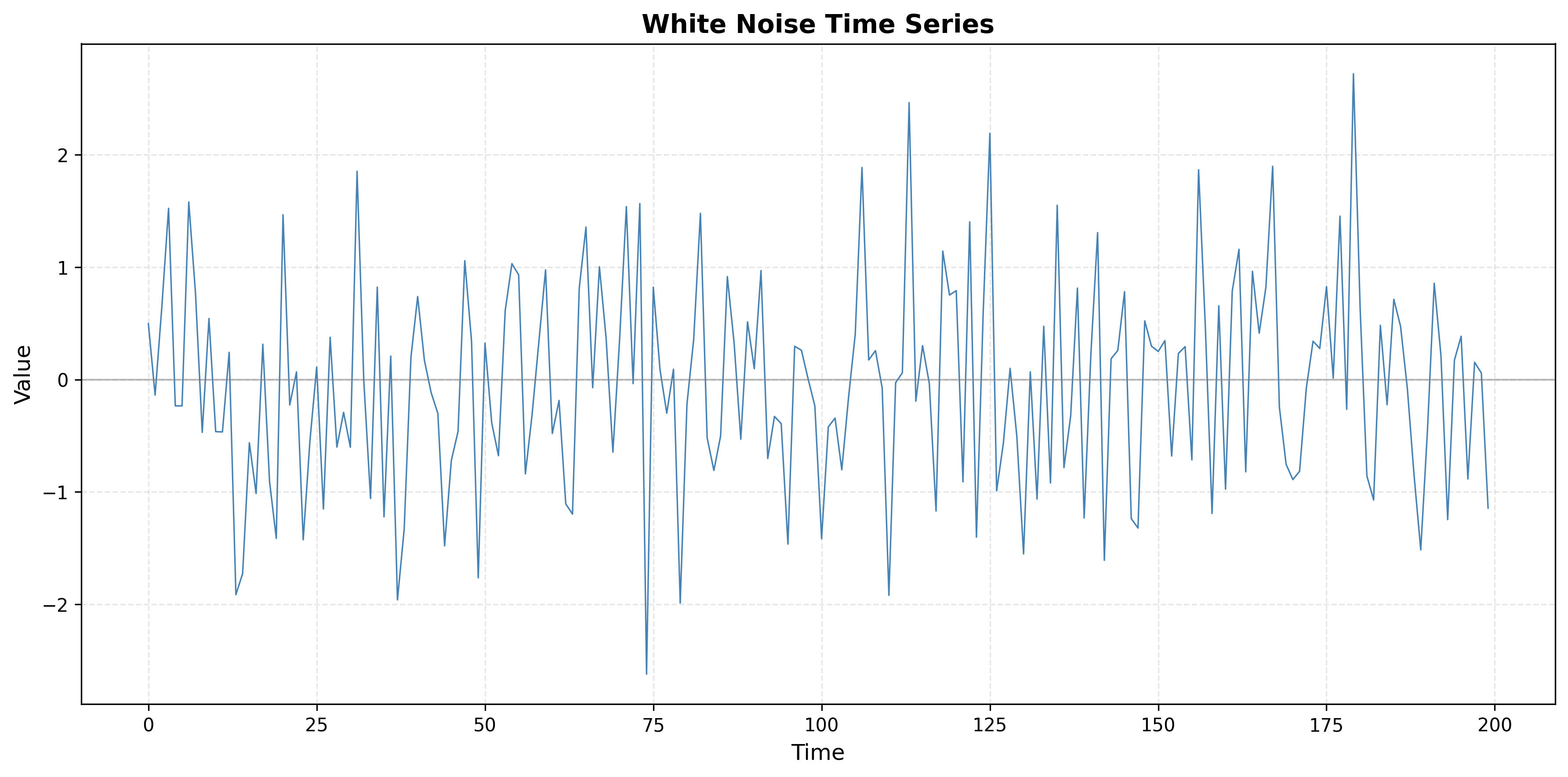
What type of process does this indicate?
What are the characteristics of such a process?
Generate a synthetic time series with this ACF pattern and plot both the series and its ACF.

Problem 3.2

A time series has an ACF plot showing ρ(k) that decays very slowly, remaining positive and significant even at large lags (e.g., ρ(20) > 0.5).

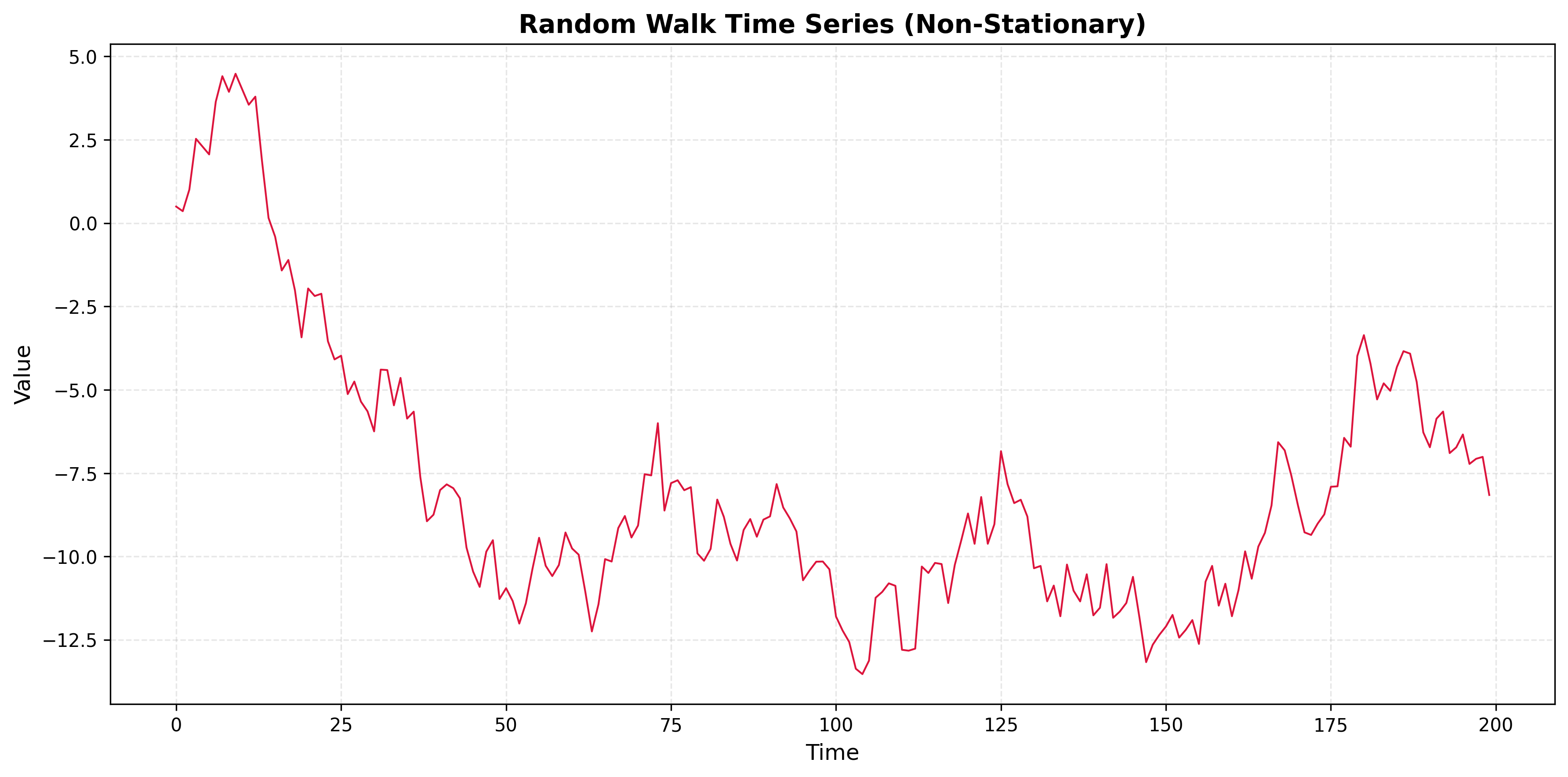
What does this pattern indicate?
What type of non-stationarity is likely present?
Generate a synthetic time series with this ACF pattern and plot both the series and its ACF.

Problem 3.3

A time series has an ACF plot showing oscillatory (sinusoidal) behavior, with autocorrelations alternating between positive and negative values in a periodic pattern.

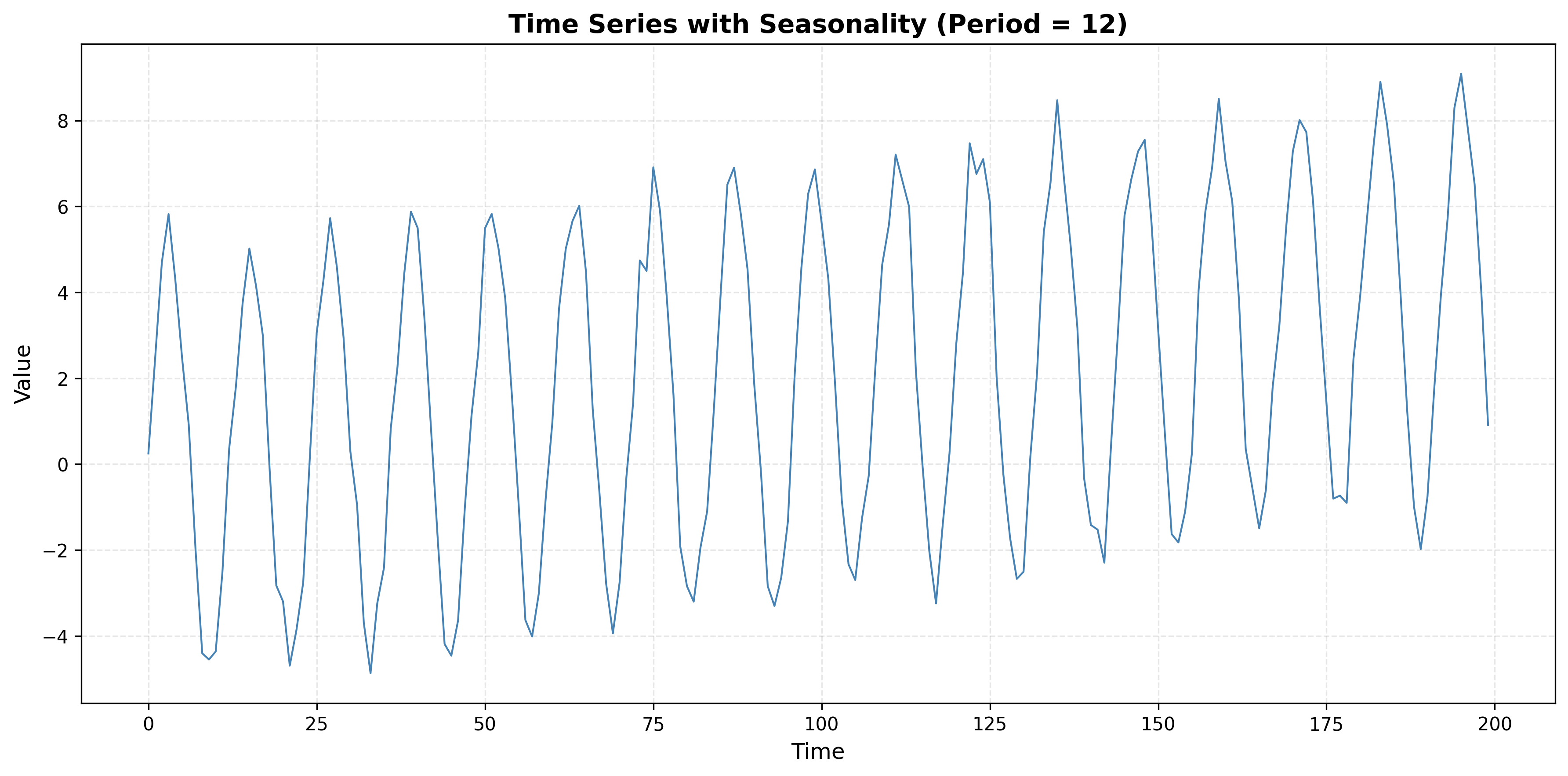
What does this pattern indicate?
What type of seasonality or cyclical behavior is present?
Generate a synthetic time series with this ACF pattern and plot both the series and its ACF.

Problem 3.4

A time series has an ACF plot where ρ(k) shows a sharp cutoff after lag q = 2, with ρ(1) and ρ(2) being significant, but ρ(k) ≈ 0 for all k > 2.

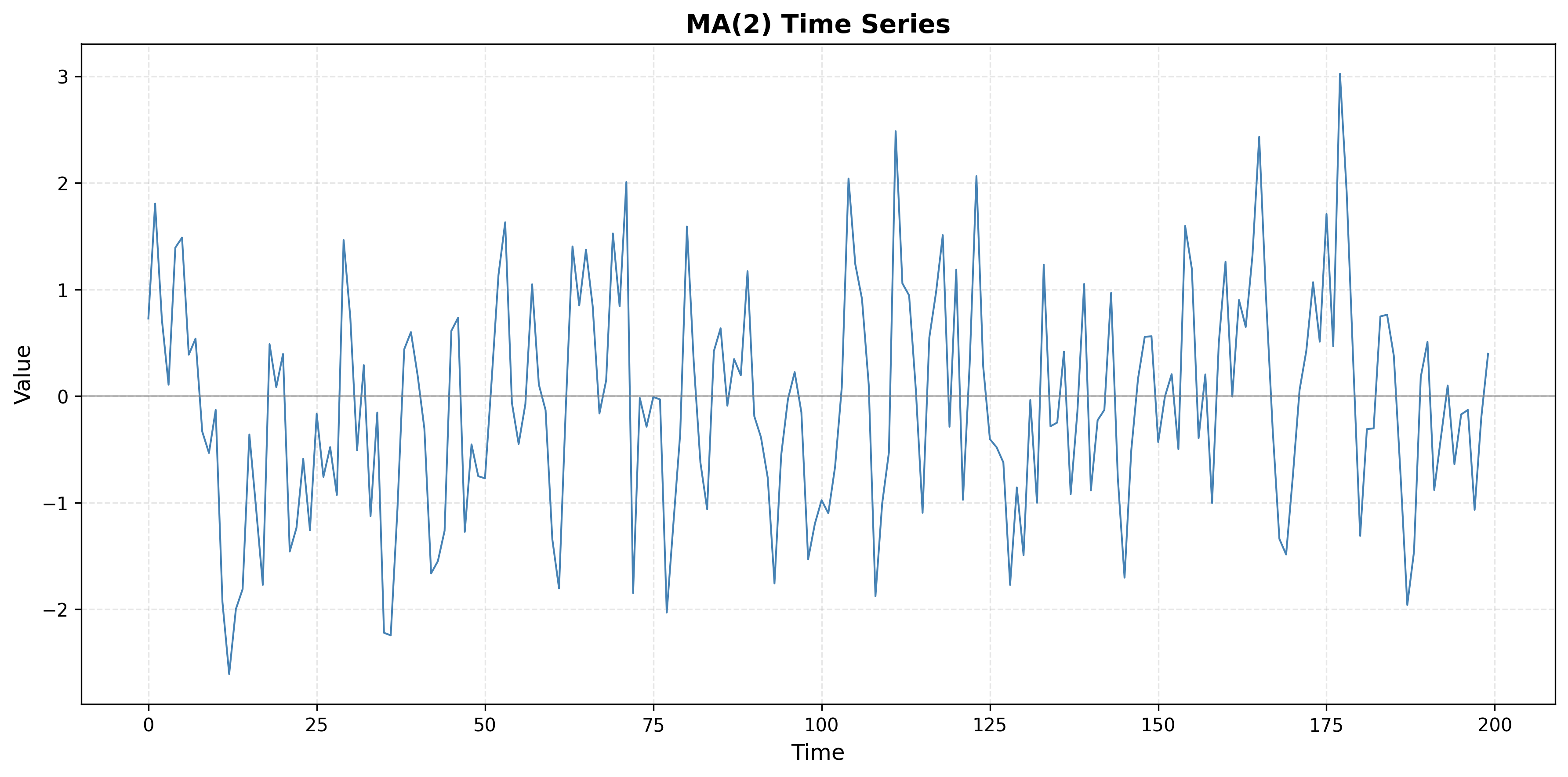
What type of process does this suggest?
What is the likely model order?
Generate a synthetic time series with this ACF pattern and plot both the series and its ACF.

Problem 3.5

A time series has an ACF plot showing exponential decay: ρ(k) starts high and decays gradually, remaining positive but decreasing, with no sharp cutoff.

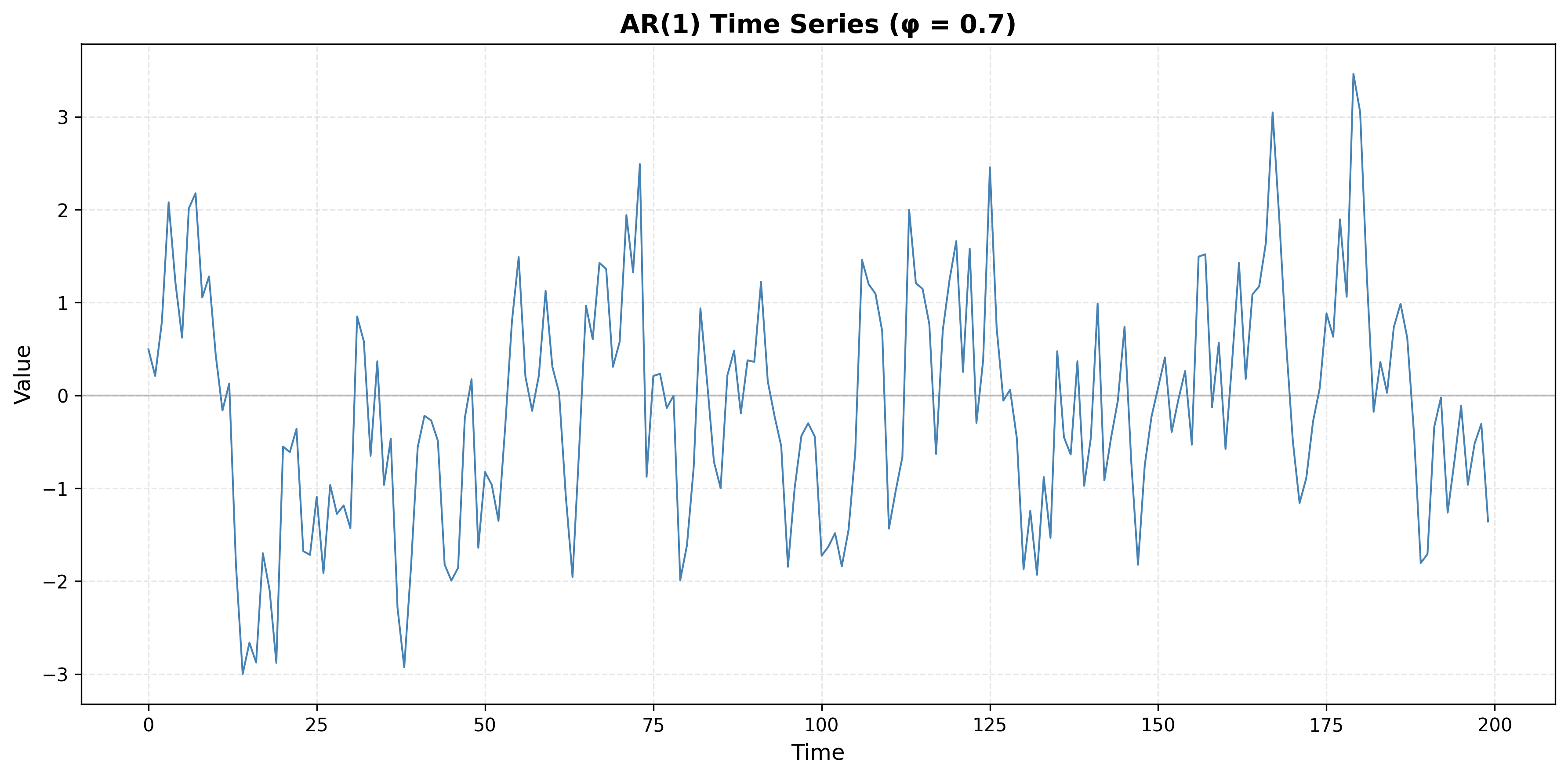
What type of process does this indicate?
How does this differ from the MA process pattern?
Generate a synthetic time series with this ACF pattern and plot both the series and its ACF.

Exercise Type 4: Physiological Time-Series Interpretation

Problem 4.1

Consider a heart rate time series where the ACF shows:

Strong positive autocorrelation at lag 1 (ρ(1) ≈ 0.8)
Rapid decay to near zero by lag 5
No significant periodic patterns

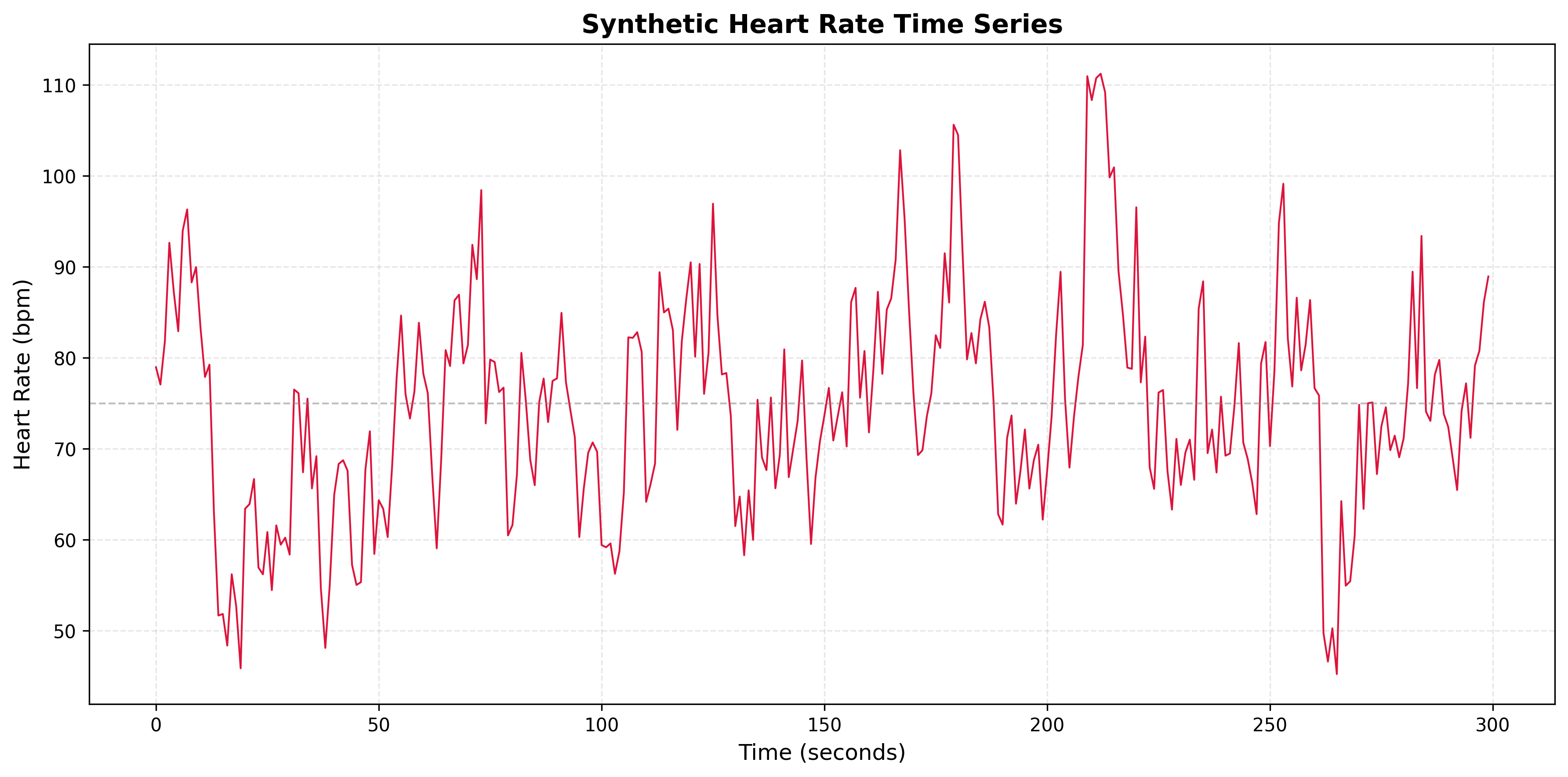
What does this tell you about the memory length of the process?
What AR/MA/ARIMA model order would be appropriate?
Would deep learning be necessary for forecasting?
Generate a synthetic heart rate time series with these characteristics and plot the series and ACF.

Problem 4.2

Consider a blood pressure time series where the ACF shows:

Very slow decay, remaining above 0.5 even at lag 20
No clear periodic pattern
Gradual decrease rather than sharp cutoff

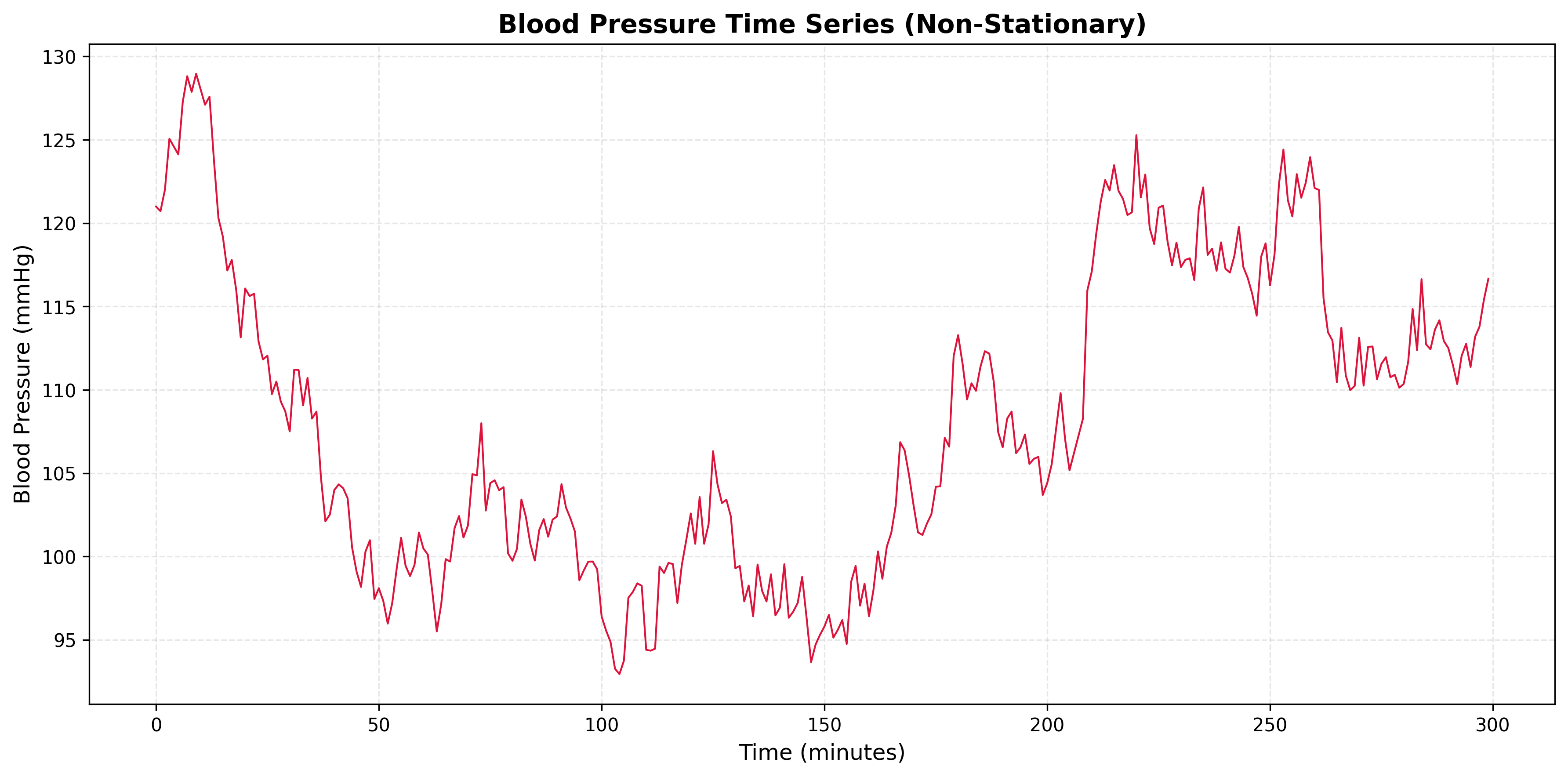
What does this indicate about the process?
What preprocessing step might be necessary?
What model would be appropriate after preprocessing?
Generate a synthetic blood pressure time series and plot the series and ACF.

Problem 4.3

Consider an EEG-like signal where the ACF shows:

Oscillatory pattern with period approximately 10 time steps
Significant autocorrelation at lags 10, 20, 30
Decay in amplitude of oscillations over time

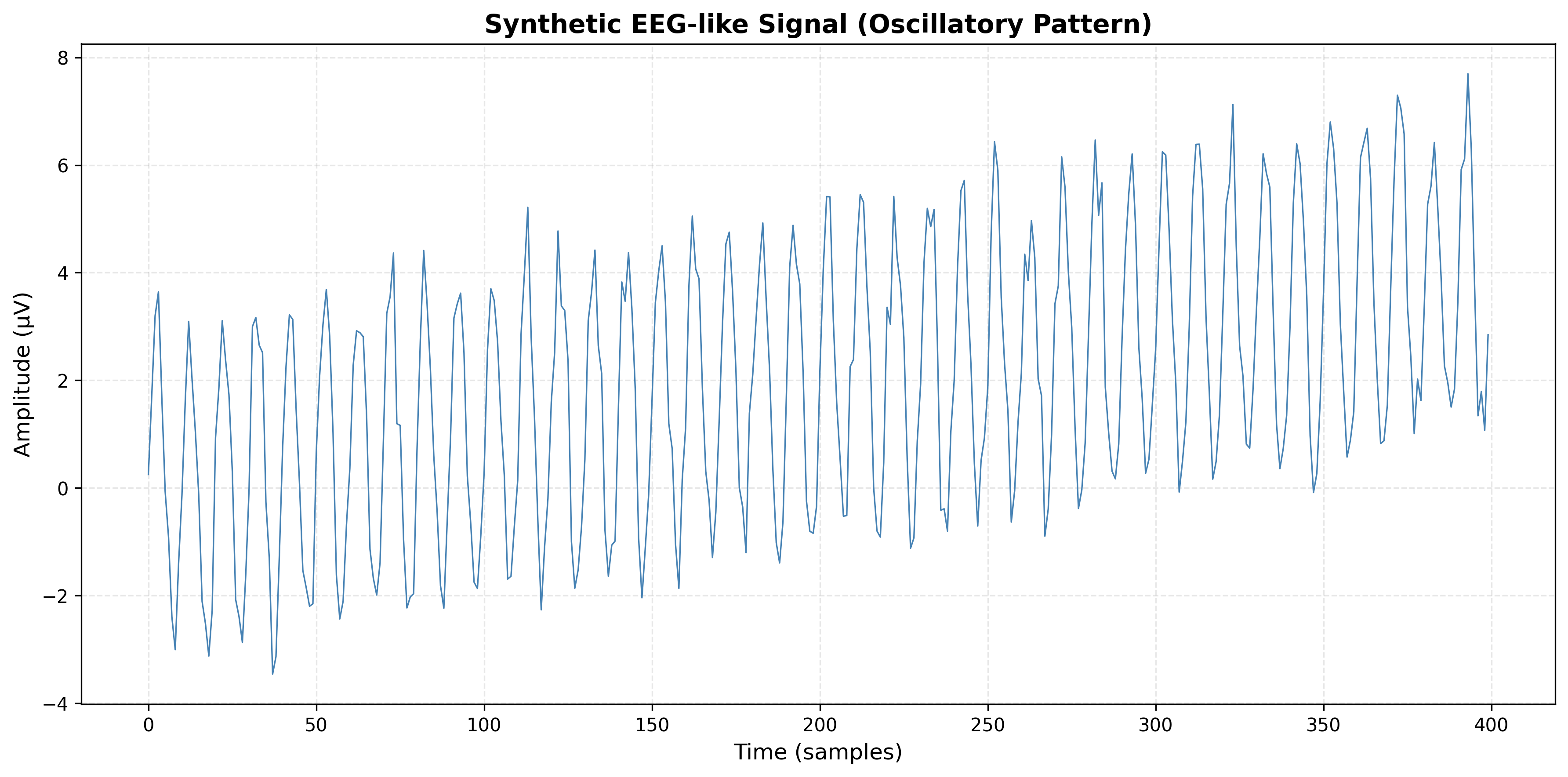
What does this indicate about the signal?
What type of seasonality is present?
Would a seasonal ARIMA model be appropriate?
Generate a synthetic EEG-like signal and plot the series and ACF.

Problem 4.4

Consider a respiratory rate time series where the ACF shows:

Sharp cutoff after lag 2
ρ(1) ≈ 0.6, ρ(2) ≈ 0.3
ρ(k) ≈ 0 for k > 2

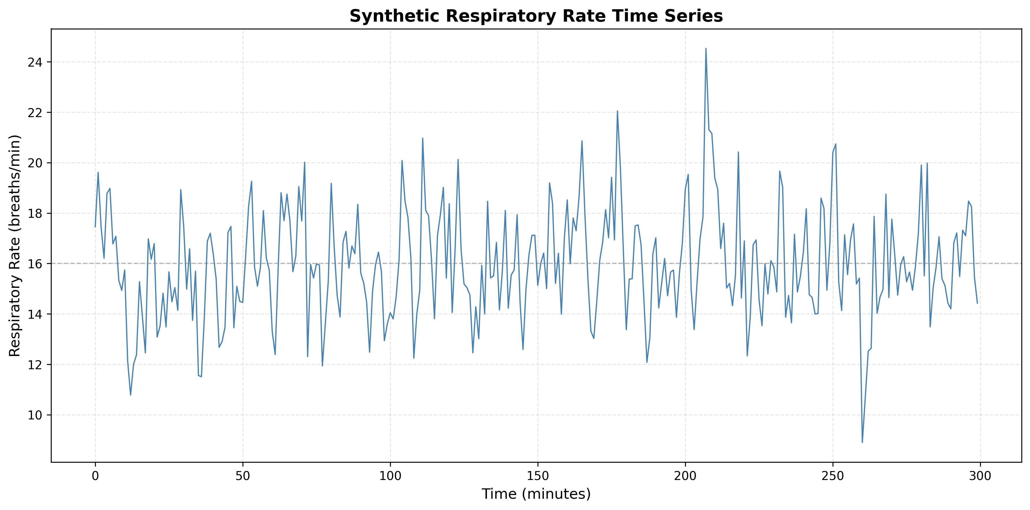
What type of process does this indicate?
What is the memory length?
What model order would be appropriate?
Generate a synthetic respiratory rate time series and plot the series and ACF.

Problem 4.5

Consider a body temperature time series where the ACF shows:

Exponential decay starting at ρ(1) ≈ 0.9
Gradual decrease: ρ(5) ≈ 0.5, ρ(10) ≈ 0.2
All values positive, no oscillations

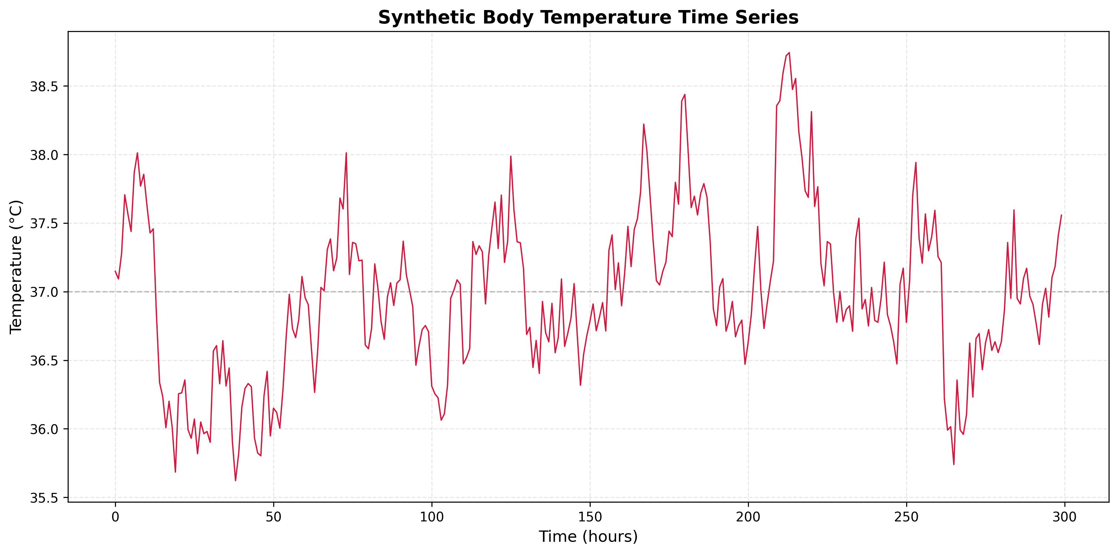
What type of process does this indicate?
What is the approximate memory length?
Would deep learning provide significant advantages over traditional methods?
Generate a synthetic body temperature time series and plot the series and ACF.

Summary

This problem set covers:

Numerical ACF Calculation: Manual computation of autocovariance and autocorrelation, including edge cases (constant series, zero variance).
Mean Removal Effect: Understanding why mean removal is essential for correct autocorrelation computation and avoiding spurious correlations.
ACF Pattern Interpretation: Identifying process types (white noise, trend, seasonality, AR, MA) from ACF plots with Python visualizations.
Physiological Time-Series: Applying ACF analysis to real-world biomedical signals, determining appropriate models, and assessing when advanced methods are needed.

This problem set provides exercises for practice. Solutions are available separately.