Airline Passenger Time Series

Level: Easy
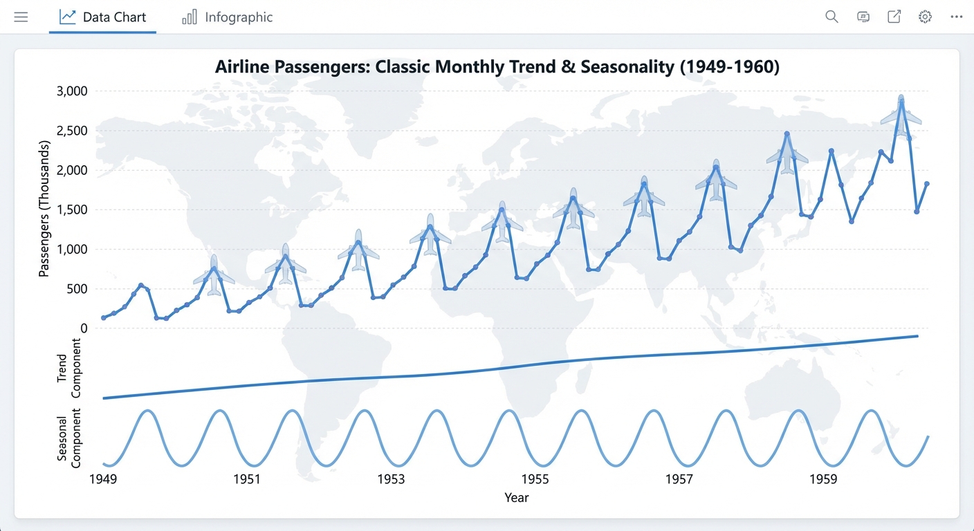
Goal: Classic monthly airline passenger series (trend + seasonality) using a library dataset.

Dataset & Library

• Dataset: AirPassengers dataset via statsmodels.datasets.get_rdataset
• Library: statsmodels

Installation

pip install statsmodels

Data Loading

import pandas as pd
from statsmodels.datasets import get_rdataset

data = get_rdataset("AirPassengers", "datasets").data
# Original data typically has a 'time' or 'Month' column and 'value' column
print(data.head())

# If there is only an index and a passenger column:
# Example conversion (adapt depending on structure)
data["Month"] = pd.date_range(start="1949-01-01", periods=len(data), freq="M")
data = data.set_index("Month").sort_index()
data.rename(columns={data.columns[0]: "Passengers"}, inplace=True)

print(data.head())

Implementation Steps

1. Data Loading and Exploration

• Load AirPassengers dataset using statsmodels
• Inspect data structure and format
• Convert to proper time series format (datetime index)
• Examine basic statistics and data range

2. Exploratory Data Analysis (EDA)

• Plot the time series (should show clear trend and seasonality)
• Identify trend (increasing over time)
• Identify seasonality (yearly pattern, peak in summer)
• Perform time series decomposition (additive or multiplicative)
• Calculate and visualize ACF/PACF plots

3. Stationarity Analysis

• Test for stationarity (ADF test) - will be non-stationary
• Apply first differencing
• Apply seasonal differencing if needed
• Test transformed series for stationarity

4. Model Building

• ARIMA Models:
  • Use ACF/PACF to identify (p, d, q)
  • Try multiple ARIMA configurations
• SARIMA Models (recommended):
  • Identify seasonal pattern (12 months)
  • Fit SARIMA models: SARIMA(p, d, q)(P, D, Q)12
  • Try different seasonal configurations
• Exponential Smoothing:
  • Holt-Winters method (additive or multiplicative)
  • Compare with ARIMA/SARIMA

5. Model Selection

• Compare models using AIC/BIC
• Use cross-validation or hold-out validation
• Select best model based on validation performance
• Check residual diagnostics

6. Model Evaluation

• Split data (e.g., last 2 years as test set)
• Generate forecasts
• Calculate accuracy metrics (MAE, RMSE, MAPE)
• Visualize forecasts with actual values
• Analyze forecast errors

7. Forecasting

• Generate future forecasts (e.g., next 12-24 months)
• Include prediction intervals
• Visualize with historical data
• Interpret results

Expected Deliverables

1. EDA Report:

   • Time series plot showing trend and seasonality
   • Decomposition plots (trend, seasonal, residual)
   • ACF/PACF plots
   • Stationarity test results

2. Model Results:

   • Best model with parameters (e.g., SARIMA(1,1,1)(1,1,1)12)
   • Model diagnostics (residual plots, ACF of residuals)
   • Forecast accuracy metrics
   • Forecast plots with confidence intervals

3. Code:

   • Complete Python notebook
   • Functions for model fitting and evaluation
   • Visualization utilities

Tips

• This is a classic dataset perfect for learning ARIMA/SARIMA
• Strong seasonality (yearly pattern) - SARIMA is highly recommended
• Multiplicative seasonality is common (variance increases with level)
• Use seasonal differencing for SARIMA models
• Compare additive vs multiplicative models
• This dataset is well-studied - results should align with literature
• Good for demonstrating Box-Jenkins methodology
• Perfect for understanding trend + seasonality decomposition